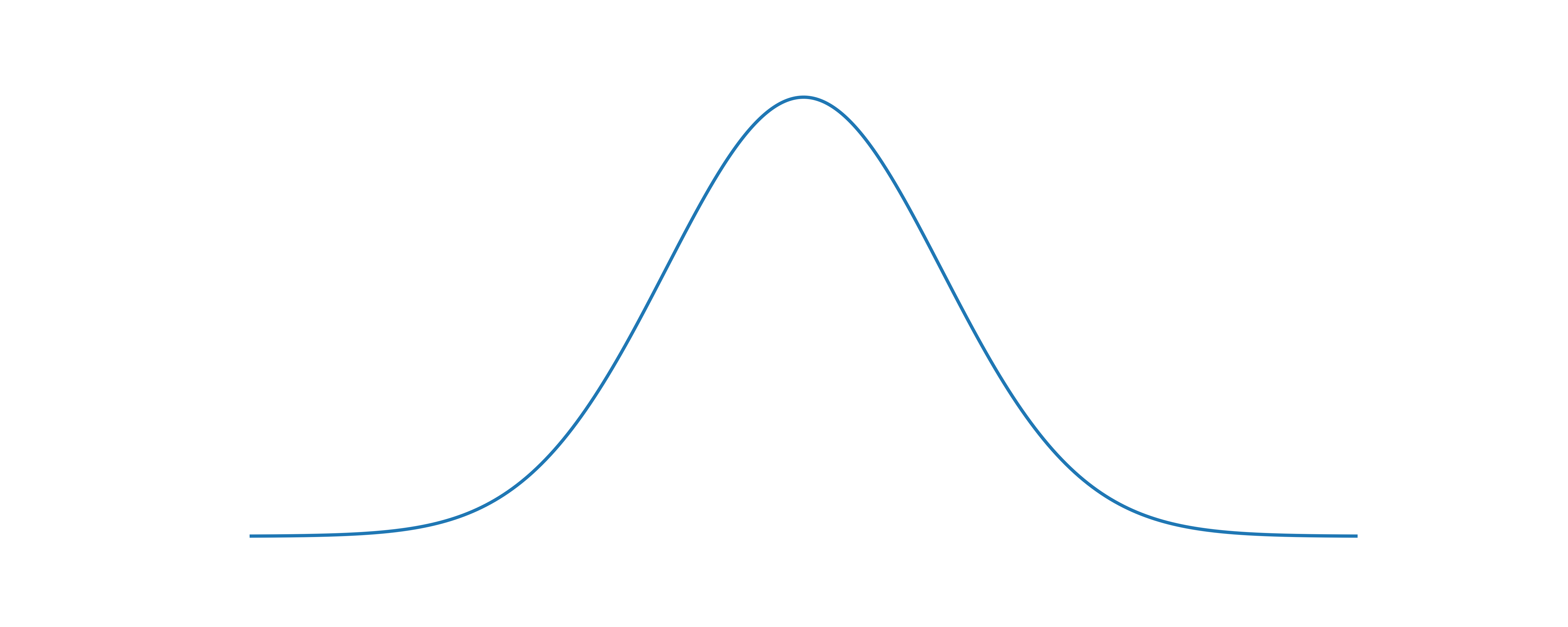
Integrating the PDF of the Normal Distribution


For my first blog post, I will demonstrate the classic integral trick to show that the pdf of the normal distribution does in fact meet the requirements of a probability density function and have integral 1.

A Double Integral

First, recall that the pdf of the normal distribution is f(x)=12πe−x22f(x)=\frac{1}{\sqrt{2\pi}}e^{-\frac{x^2}{2}} . This function does not yield to integration by parts or substitution, and so a trick is necessary.

Let

I=∫−∞∞12πe−x22dxI=\int_{-\infty}^\infty\frac{1}{\sqrt{2\pi}}e^{-\frac{x^2}{2}}dx

Observe that II is always positive, because the integrand is always positive. Hence, to show that II is equal to 1, it is enough to show that I2I^2 is equal to 1.

Polar Coordinates

Consider the following:

I2=∫−∞∞f(x)dx⋅∫−∞∞f(y)dyI^2=\int_{-\infty}^{\infty}f(x)dx\cdot\int_{-\infty}^{\infty}f(y)dy
Because the second integral is a constant with respect to xx , it is reasonable to move it inside the integral sign:

I2=∫−∞∞∫−∞∞f(x)f(y)dydx=∫−∞∞∫−∞∞12πe−x2+y22dydx\begin{align*}I^2&=\int_{-\infty}^{\infty}\int_{-\infty}^{\infty}f(x)f(y)dydx\\ &=\int_{-\infty}^{\infty}\int_{-\infty}^{\infty}\frac{1}{2\pi}e^{-\frac{x^2+y^2}{2}}dydx\end{align*}

Consider the following parameterization of xx and yy :

let

x↦rcos⁡θy↦rsin⁡θ\begin{align*} x &\mapsto r\cos\theta\\ y &\mapsto r\sin\theta \end{align*}

which is the standard change to polar coordinates. The integral can be computed in these new coordinates, by the change of variables theorem.

I2=∫02π∫0∞12πe−r22∣∂(x,y)∂(r,θ)∣drdθ=∫02π∫0∞12πe−r22∣∂x∂r∂x∂θ∂y∂r∂y∂θ∣drdθ=∫02π∫0∞12πe−r22∣cos⁡θ−rsin⁡θsin⁡θrcos⁡θ∣drdθ=∫02π∫0∞12πe−r22(sin⁡2θ+cos⁡2θ)rdrdθ=∫02π∫0∞12πe−r22rdrdθ\begin{align*} I^2&=\int_{0}^{2\pi}\int_0^\infty \frac{1}{2\pi}e^{-\frac{r^2}{2}}\left| \frac{\partial(x, y)}{\partial(r, \theta)} \right|drd\theta\\ &= \int_{0}^{2\pi}\int_0^\infty \frac{1}{2\pi}e^{-\frac{r^2}{2}} \begin{vmatrix} \frac{\partial x}{\partial r} & \frac{\partial x}{\partial \theta} \\ \frac{\partial y}{\partial r} & \frac{\partial y}{\partial \theta} \end{vmatrix}drd\theta \\ &= \int_0^{2\pi}\int_0^\infty \frac{1}{2\pi}e^{-\frac{r^2}{2}} \begin{vmatrix} \cos\theta & -r\sin\theta \\ \sin\theta & r\cos\theta \end{vmatrix}drd\theta \\ &= \int_0^{2\pi} \int_0^\infty \frac{1}{2\pi}e^{-\frac{r^2}{2}}\left(\sin^2\theta+\cos^2\theta\right)rdrd\theta \\ &= \int_0^{2\pi}\int_0^\infty\frac{1}{2\pi} e^{-\frac{r^2}{2}}rdrd\theta \end{align*}

Completing the integral

The key point to notice is that the transition from dxdydxdy to rdrdθrdrd\theta allows us to use substitution to compute the integral.

Let u=−r22,du=−rdru=-\frac{r^2}{2}, du=-rdr and notice that

I2=∫02π∫0−∞−12πeududθ=∫02π12π(1−0)dθ=1\begin{align*} I^2&=\int_{0}^{2\pi}\int_0^{-\infty} -\frac{1}{2\pi}e^{u}dud\theta \\ &= \int_0^{2\pi} \frac{1}{2\pi} (1-0) d\theta \\ &= 1 \end{align*}

and so the pdf of the normal distribution is shown to have integral 1 as desired. This is a classic fun integral trick that is worth knowing, and it applies for all means and variances (above is the mean 0 and variance 1 case). Probability as a field often results in enjoyable integrals.